Setting up a cruise - Allowable Error

When you plan a cruise, you’re usually planning to answer a specific question - how much merchantable material would come out if I thinned this stand?  Is stocking high enough for a selection harvest?  Should I buy/sell this property?  How much is this tract worth?

When setting up a cruise on SilviaTerra.com, the number of plots in a cruise depends on the level of confidence you want in the answers, and the amount of error in the estimates you decide is acceptable. How do you go about choosing what error and confidence you prefer?  To answer that question, you might ask yourself another: how much does it cost you if your cruise answers your question “incorrectly"?

If you try changing the values for confidence and error, you can see that decreasing confidence and increasing error both result in fewer plots in the cruise layout, and increasing confidence or decreasing error results in more plots. The allowable error is the precision you require for your final stocking estimates.  The confidence is the probability that your final estimate ± a confidence interval contains the true mean for the stand (what you would get if you measured every single tree).

          

There is a tradeoff between the cost of measuring plots and the cost if your estimate is “wrong”. Measuring plots also costs you both time and money.  Consider an example of a 100 acre stand with an estimated variation of 0.25. 

Plots	Cost to cruise ($50/plot)	Confidence	Allowable Error
17	$850	0.9	0.1
5	$250	0.9	0.2
2	$100	0.9	0.3

We’ll assume a stumpage price of $100/MBF.

If the merchantable volume in the stand is 5000 board feet of sawtimber per acre, then the “true” value of the stand is 5 MBF * $100/MBF, or  $500 per acre. That becomes $50,000 for the 100-acre stand.

If your allowable error is 0.1, and your plots are accurate, perhaps your estimated volume would be 4600 board feet (± 460); or, 5400 board feet ± 540.  Scaled out, that could put your estimate of value anywhere from $46,000 to $54,000, with your estimate still falling within the allowable error you specified at the beginning.

But suppose you specified an allowable error of 0.2.  Installing 5 plots would be faster and easier than putting in 17, but your estimated volume could be anywhere from 4200 bd ft to 7500 bd ft.  Your final estimated value could range from $42,000 to $75,000. 

So in this case, if estimating a value of $75K for a stand worth $50K would be acceptable for your purposes, a 20% (0.2) allowable error would be a reasonable choice.  But the “cost” of being wrong would be $25,000; the cost of putting in plots to meet an acceptable error of 0.1 would only be an additional $600.

If measurements from 17 plots and from 4 plots both resulted in an average of 5000 board feet per acre, that would be a value reported as either 5000 ± 1000 board feet, or, 5000 ± 500 board feet.  You can see that the price of that precision is $650.

It’s important to consider the tradeoffs of time spent cruising and the precision and confidence in your results. Keep this in mind when you select the acceptable error and confidence for the next cruise you design!

Setting up a cruise - Estimating Variation

Measuring plots, from a birds-eye view, probably looks a little absurd.  You head for a very specific spot on the ground in the middle of the woods, and that is the “right spot” to begin measurements.  It’s weird to think that going to one particular point is valid, but just a few feet away would bias your sample.  However, we set up your cruise so that it’s important to visit that specific patch of woods and take measurements there, and then move on to the next location. 

So, how do you know where to go?

One approach to designing a cruise is to specify an acceptable level of confidence and error, collect data, and calculate the variance and standard error in the field as you sample.  If variance is too high, you keep adding plots until you reached an acceptable level.  This is somewhat inconvenient, though- it requires you to perform calculations on-the-fly in the woods, and it’s hard to anticipate when you’ll be done cruising on a given day, or in a given stand.  It can also be inefficient, if you add new random plot locations and have to criss-cross the property multiple times.

An alternate approach is to estimate the variation before you enter the stand, and design your cruise accordingly.  That’s the method we employ when you design a new cruise for Plot Hound. Plots are automatically generated along a grid across the stand, and you’ve probably noticed that changing the criteria you specify for variation, confidence, and error changes the sampling design.

Of these criteria, one of the critical decisions you make is your estimate of the variation within the stand.  The estimated variation is where your skill as a forester is really important.  Your familiarity with the forest type and area where the stand is located give you the knowledge you need to make that estimate.  We’re also going to start including your estimated and the actual variation in your reports, to help you “calibrate” your estimates over time.   When estimating variation, also keep in mind the size of the plots you intend to use. On average, there will be less variation between larger (fixed-area) plots than smaller ones.  

The estimated variation options we offer range from 0.15 to 0.55 - even a seemingly uniform conifer plantation or aspen stand has some variation, which is why the lowest possible value is 0.15.

For example, if you knew you were visiting a uniform plantation, like this one:

  

You might safely select a low estimated variation, maybe 0.15.

But if you knew that that plantation had experienced heavy mortality, or had a range of soil conditions, you would reasonably expect that there would be a more variation between plots, and more plots would be needed to characterize the range of structure within the stand- then you would select a higher variation.

For example, these two pictures are both taken from the same stand.  There is obviously very high variability within the stand, which would lead to high variation in stocking estimates between plots in these two locations.  More plots would be needed to reach an acceptable level of variance among all plots.

 Photo credit: Travis Pond, 2010

In upcoming posts, we’ll go into more detail on the implications of selecting the confidence and error values that also contribute to the cruise you design.

Maps are Back!

Since switching over to the new site design earlier this year, one of the top requests has been to bring back the maps.  We're happy to announce that the maps are back!

When you go to the Stands or Cruises pages, you'll now see a beautiful big map with markers for each of your stands.  The list of your stands or cruises is now located just a bit farther down below the map.

The new Stands page shows each of your stands on a map

We added a map view to the Cruises page too

Search by Address

Creating stands just got even easier.  Type an address.  Zoom to that location on the map.  We have the technology!

Today we're happy to announce that one of your top feature requests is now live.  When you go to the "Create Stand" page, you'll now see a magnifying glass in the top right of the map.  Click on it and then type the address that you want to go to.  Then hit enter and the map will zoom to that location.

Type the address in the new search bar (top right) and hit enter

The map will take you straight there!  

Then draw your stand and you're good to go

We're always working to make Plot Hound better.  Stay tuned for more improvements soon!

New Graphs: Confidence Intervals

In this blog post we’re going to explain how a confidence interval is calculated, and show some examples of data that lead to very wide or very narrow confidence intervals. We hope this will help you understand and interpret both the lines on the graphs and the composition of the stands you measure and manage. The graphs we create as part of your free basic report in Plot Hound are a summary of the plots you measured within the stand. The confidence intervals on the graphs reflect the variation between the plots for each species and each size class.

Plot	Spp	DBH
		2	4	6	8	10	12	14	16	18	20	22
1	SM	20	16	10	8	6	4	4	2	2	4	2
2	SM	30	24	15	12	9	6	6	3	3	6	3
3	SM	30	24	15	12	9	6	6	3	3	6	3
4	SM	10	8	5	4	3	2	2	1	1	2	1
5	SM	40	32	20	16	12	8	8	4	4	8	4

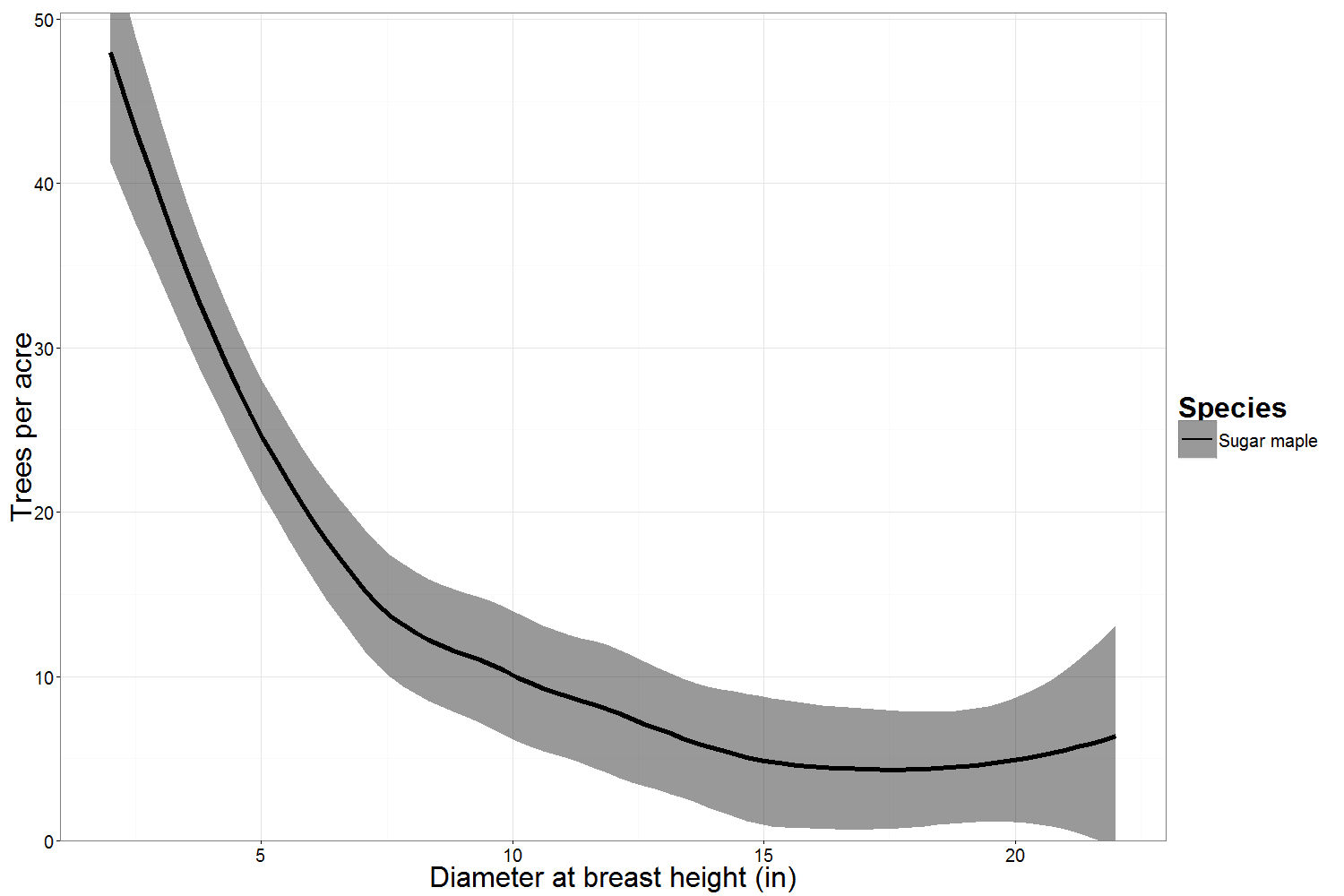
Confidence intervals reflect the standard error of the average value. For a graph like the one above, the solid line is the average number of sugar maples per acre from all the plots measured. 

We're using a 90% confidence level to determine the confidence interval in these graphs. That means that if you sampled this stand 100 times, you would expect your estimates to fall within the confidence interval above 90 of those 100 times.

We calculate the width of confidence interval by multiplying the standard error (the standard deviation of the mean, divided by the square root of the number of plots) by a statistic (the t-statistic) that is determined by the confidence level we chose.  

So we have two ways of making our confidence interval narrower. One way is to decrease our confidence level. The other is to sample more plots. A 95% confidence level would make the t-statistic larger and the confidence intervals wider; an 80% confidence interval would make the t-statistic smaller and the confidence intervals narrower. However, decreasing the confidence increases the probability that our confidence intervals do not contain the true mean of the population. If more plots are sampled, generally speaking, the confidence interval shrinks. 

- - -

You can control the confidence level and the number of plots, but there's another factor that influences the width of the confidence interval... the "standard deviation" (the variability between plots).

In the example above, all of the plots had differing numbers of trees of each diameter. Suppose that instead, all of the plots had the exact same number of trees measured in each diameter:

Plot	Spp	DBH
		2	4	6	8	10	12	14	16	18	20	22
1	SM	20	16	10	8	6	4	4	2	2	4	2
2	SM	20	16	10	8	6	4	4	2	2	4	2
3	SM	20	16	10	8	6	4	4	2	2	4	2
4	SM	20	16	10	8	6	4	4	2	2	4	2
5	SM	20	16	10	8	6	4	4	2	2	4	2

You can see that the confidence intervals are much narrower.  The variance between plots is actually zero in this example, but the confidence intervals are still present because of the smoothing function used in the graph.

We can also see how the graph changes if one plot is very different from the others.  Let’s take the first example plot, but say that no trees were measured in Plot 1, and twice as many were measured in Plot 5.

Now suppose there are twice as many plots in the sample:

Plot	Spp	DBH
		2	4	6	8	10	12	14	16	18	20	22
1	SM	20	16	10	8	6	4	4	2	2	4	2
2	SM	30	24	15	12	9	6	6	3	3	6	3
3	SM	30	24	15	12	9	6	6	3	3	6	3
4	SM	10	8	5	4	3	2	2	1	1	2	1
5	SM	40	32	20	16	12	8	8	4	4	8	4
6	SM	20	16	10	8	6	4	4	2	2	4	2
7	SM	30	24	15	12	9	6	6	3	3	6	3
8	SM	30	24	15	12	9	6	6	3	3	6	3
9	SM	10	8	5	4	3	2	2	1	1	2	1
10	SM	40	32	20	16	12	8	8	4	4	8	4

Note that plots 6-10 are the same as plots 1-5, but the confidence interval is smaller because the overall sample includes more data.

- - -

In all of these examples, we’ve been modifying the distribution of one species.  Let’s look at one more example with two species, one common to all plots and one only found in a few plots:

Plot	Spp	DBH
		2	4	6	8	10	12	14	16	18	20	22
1	SM	20	16	10	8	6	4	4	2	2	4	2
1	YB	0	0	0	0	0	0	0	0	12	0	0
2	SM	30	24	15	12	9	6	6	3	3	6	3
2	YB	0	0	0	0	0	0	0	0	0	0	0
3	SM	30	24	15	12	9	6	6	3	3	6	3
3	YB	0	0	0	0	0	0	0	0	12	0	0
4	SM	10	8	5	4	3	2	2	1	1	2	1
4	YB	0	0	0	0	0	0	0	0	0	0	0
5	SM	40	32	20	16	12	8	8	4	4	8	4
5	YB	0	0	0	0	0	0	0	0	0	0	0

As you can see, the yellow birch diameter distribution shows up in a different color and style.  As more and more species are added, there is an increasing diversity of colors and styles to differentiate them.  The same reasoning we applied above holds for interpreting the yellow birch confidence interval.

By now you should have a good sense for how the confidence level, number of plots, and stand variability influence your confidence intervals.  Be on the lookout for upcoming posts about sampling and statistics!